Mapping spatial datasets

library(inspercidados)
library(dplyr)
library(sf)
library(ggplot2)

Between 2022 and 2025, São Paulo painted faixas azuis, lanes reserved for motorcyclists, along a set of arterial corridors. Insper Cidades studied the program and deposited three datasets: a spatial layer, another spatial layer with crash counts, and a large plain table. Between them they cover most of what this package does. The article stops at describing the data. The findings belong to the study, and open_project() at the end takes you there.

All three datasets belong to one project, so filtering list_datasets() by project returns them together.

list_datasets(project = "faixa_azul")
#> # A tibble: 3 × 11
#>   alias         title description theme region project access is_spatial formats
#>   <chr>         <chr> <chr>       <chr> <chr>  <chr>   <chr>  <lgl>      <chr>  
#> 1 faixa_azul_sp Trec… Localizaçã… Mobi… São P… faixa_… downl… TRUE       geojso…
#> 2 sinistros_sp  Sini… Sinistros … Mobi… São P… faixa_… downl… FALSE      parque…
#> 3 sinistros_vi… Sini… Localizaçã… Mobi… São P… faixa_… downl… TRUE       geojso…
#> # ℹ 2 more variables: keywords <chr>, doi <chr>

Download the lanes

list_resources() reports what an alias contains before anything is downloaded. faixa_azul_sp holds one resource in three formats.

list_resources("faixa_azul_sp")
#> # A tibble: 1 × 6
#>   resource title      is_spatial years formats                default
#>   <chr>    <chr>      <lgl>      <chr> <chr>                  <lgl>  
#> 1 dados    Faixa Azul TRUE       NA    geojson, gpkg, parquet TRUE

get_dataset() downloads it. Spatial resources come back as sf objects, so the layer arrives ready to map.

lanes <- get_dataset("faixa_azul_sp", format = "gpkg")

glimpse(st_drop_geometry(lanes))
#> Rows: 1,047
#> Columns: 16
#> $ id_osm                    <chr> "4328549", "4330744", "4331361", "4331371", …
#> $ logradouro                <chr> "Avenida das Nações Unidas", "Avenida Washin…
#> $ logradouro_alt1           <chr> NA, NA, NA, NA, NA, NA, NA, NA, NA, NA, "Ave…
#> $ logradouro_alt2           <chr> NA, NA, NA, NA, NA, NA, NA, NA, NA, NA, NA, …
#> $ logradouro_alt3           <chr> NA, NA, NA, NA, NA, NA, NA, NA, NA, NA, NA, …
#> $ logradouro_ref            <chr> "SP-015", NA, NA, NA, NA, NA, NA, NA, NA, NA…
#> $ tipo_via                  <chr> "trunk", "trunk", "trunk", "trunk", "trunk",…
#> $ faixas                    <chr> "3", "3", "3", "3", "3", "3", "4", "4", "4",…
#> $ limite_velocidade         <chr> "60", "50", "60", "50", "60", "60", "50", "5…
#> $ limite_velocidade_pesados <chr> "50", NA, NA, NA, NA, NA, NA, NA, NA, NA, NA…
#> $ motocicleta               <chr> NA, NA, NA, NA, NA, NA, NA, NA, NA, NA, NA, …
#> $ mao_unica                 <chr> "yes", "yes", "yes", "yes", "yes", "yes", "y…
#> $ superficie                <chr> "asphalt", "asphalt", "asphalt", "asphalt", …
#> $ elevado                   <chr> NA, NA, NA, NA, NA, NA, "yes", NA, NA, NA, N…
#> $ comprimento               <dbl> 645.74847, 58.75908, 448.52227, 161.48188, 4…
#> $ data_implementacao        <date> 2023-11-01, 2024-04-01, 2023-10-01, 2024-04…

Each row is one painted segment, with the street it sits on, the road attributes around it, and data_implementacao, the month the paint went down.

sinistros_via_sp covers the road segments the study analyzed. Its geometry makes a useful backdrop for the lanes.

roads <- get_dataset("sinistros_via_sp", format = "gpkg")

Drawing one layer over the other shows where the lanes run.

ggplot() +
  geom_sf(data = roads, colour = "grey80", linewidth = 0.25) +
  geom_sf(data = lanes, colour = "#1D4ED8", linewidth = 0.8) +
  labs(
    title = "Motorcycle lanes in São Paulo",
    subtitle = "Segments painted between 2022 and 2025"
  ) +
  theme_void()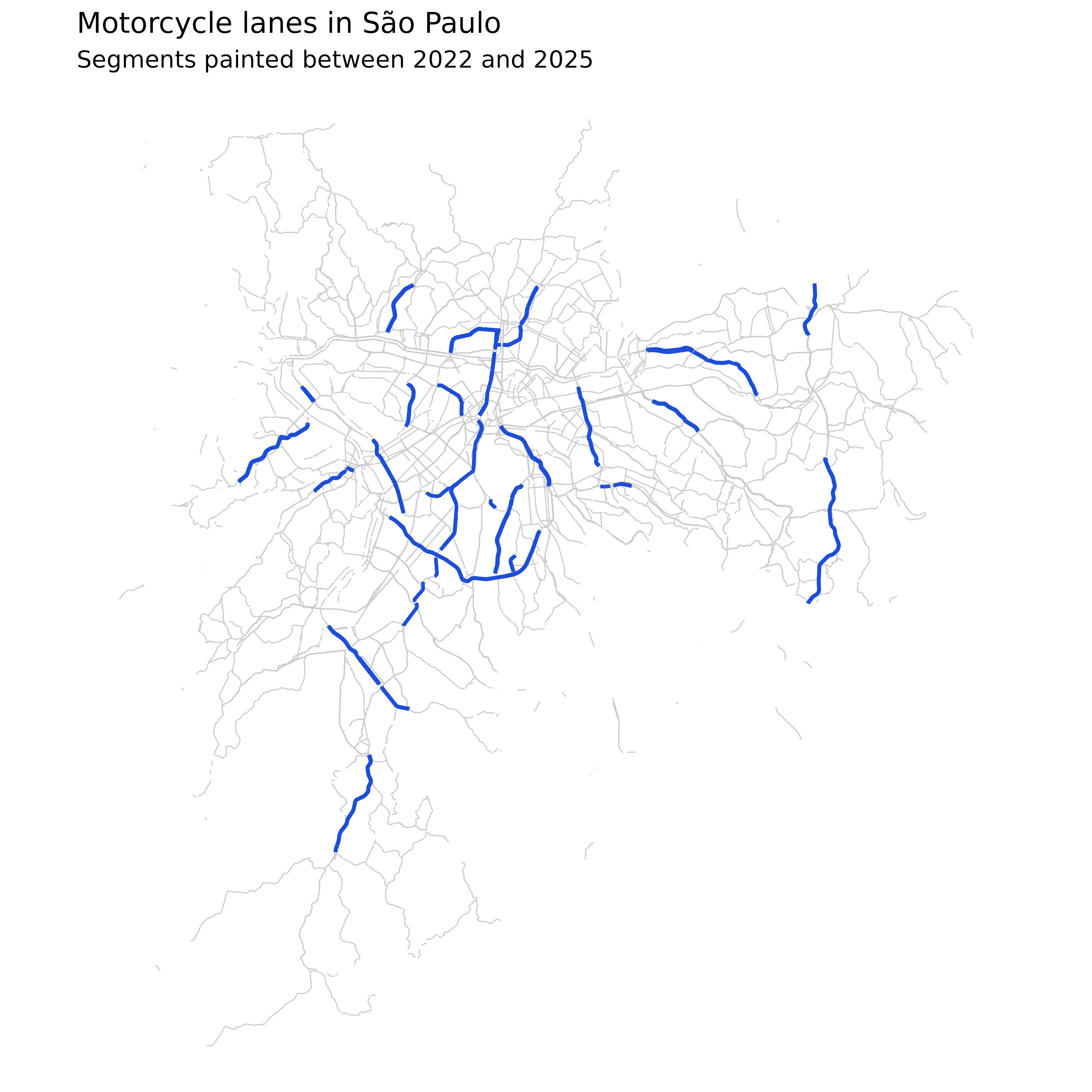

Map of São Paulo showing the road segments in the study as faint gray lines, with the motorcycle lanes drawn in blue on top. The blue corridors are scattered across the city, several of them radiating from the center.

data_implementacao dates each segment, so the same layer doubles as a timeline.

lanes <- lanes |>
  mutate(year = format(data_implementacao, "%Y"))

lanes |>
  st_drop_geometry() |>
  as_tibble() |>
  summarise(
    segments = n(),
    km = sum(comprimento, na.rm = TRUE) / 1000,
    .by = year
  ) |>
  arrange(year)
#> # A tibble: 4 × 3
#>   year  segments     km
#>   <chr>    <int>  <dbl>
#> 1 2022       102  21.3 
#> 2 2023       363  71.2 
#> 3 2024       571 120.  
#> 4 2025        11   2.01

ggplot() +
  geom_sf(data = roads, colour = "grey85", linewidth = 0.2) +
  geom_sf(data = lanes, aes(colour = year), linewidth = 0.8) +
  scale_colour_viridis_d(
    option = "mako",
    end = 0.8,
    direction = -1,
    name = NULL
  ) +
  labs(title = "Motorcycle lanes by year of implementation") +
  theme_void()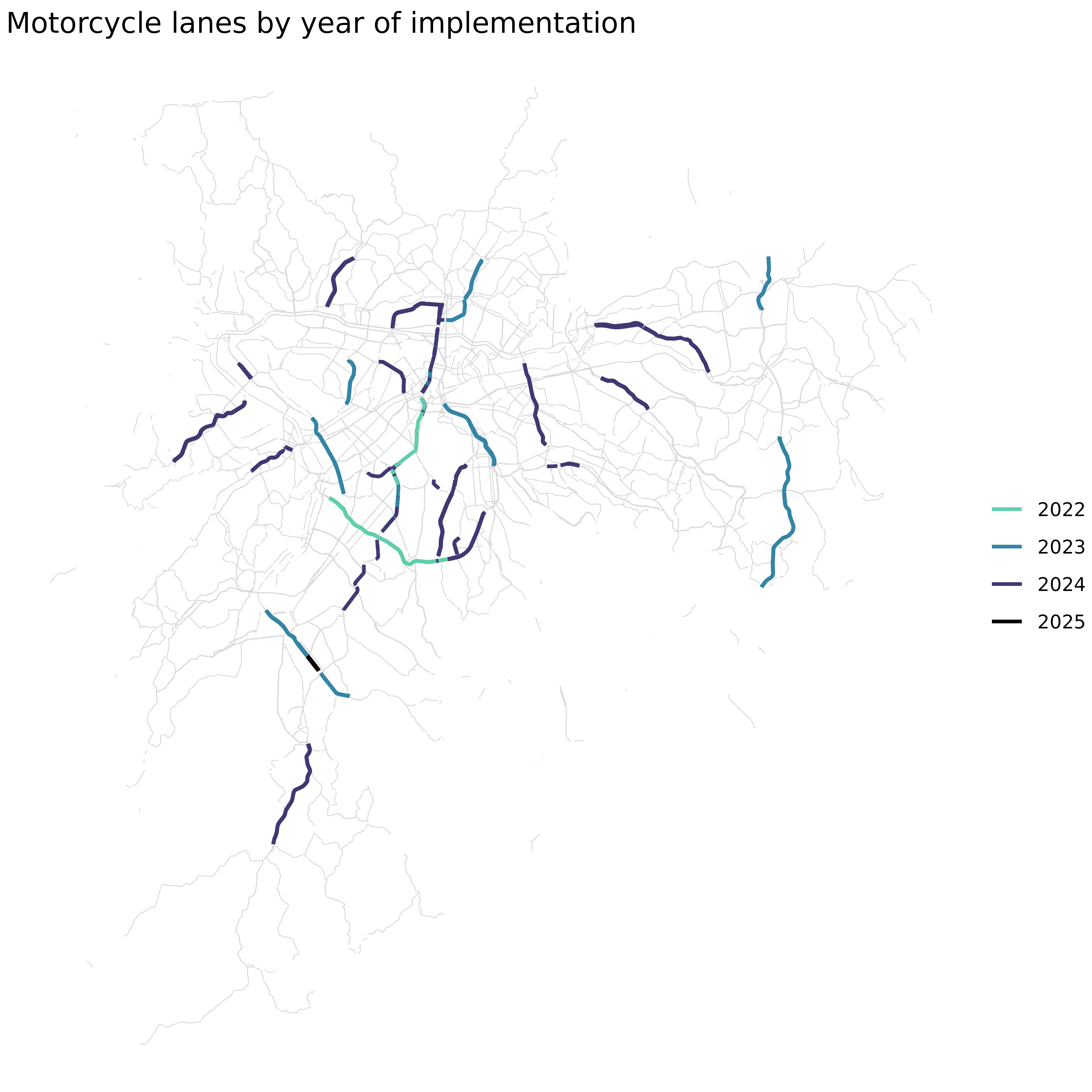

The same map of motorcycle lanes, now colored by the year each segment was painted, running from green in 2022 through blue and purple to black in 2025.

Read the attributes and the crash table

sinistros_via_sp is the same kind of object as the lanes, with crash counts attached to each segment.

glimpse(st_drop_geometry(roads))
#> Rows: 5,068
#> Columns: 26
#> $ id_trecho_agregado   <chr> "00002-000-000", "00004-000-000", "00007-000-000"…
#> $ trechos              <dbl> 2, 2, 2, 4, 7, 3, 2, 3, 6, 4, 5, 5, 2, 2, 1, 1, 3…
#> $ comprimento          <dbl> 393.9379, 243.9870, 236.2866, 426.4570, 404.5975,…
#> $ data_implementacao   <date> NA, NA, NA, NA, NA, NA, NA, NA, NA, NA, NA, NA, …
#> $ faixas               <dbl> 2.000000, 2.000000, 2.000000, 2.000000, 2.142857,…
#> $ limite_velocidade    <dbl> 50, NA, 50, 50, 50, NA, NA, 40, NA, NA, 40, 40, 5…
#> $ amenidades           <dbl> 2, 2, 2, 4, 7, 3, 3, 3, 6, 4, 5, 5, 2, 2, 1, 2, 8…
#> $ intersec             <dbl> 14, 8, 8, 10, 16, 10, 9, 32, 13, 15, 6, 3, 11, 17…
#> $ tipo_via             <chr> "trunk", "secondary", "secondary", "secondary", "…
#> $ radar_proximo        <dbl> 1, 0, 0, 0, 0, 0, 0, 0, 0, 0, 0, 0, 0, 0, 0, 1, 1…
#> $ mao_unica            <chr> "yes", "yes", "yes", "no", "no", "yes", "yes", NA…
#> $ superficie           <chr> NA, "asphalt", "asphalt", "asphalt", "asphalt", "…
#> $ total_sinistros      <int> 1, 0, 8, 9, 4, 1, 4, 10, 12, 47, 8, 0, 2, 2, 4, 6…
#> $ sinistros_fatal      <int> 0, 0, 0, 0, 0, 0, 0, 0, 1, 1, 0, 0, 0, 0, 1, 0, 0…
#> $ atropelamento        <int> 0, 0, 2, 1, 0, 0, 2, 4, 1, 7, 1, 0, 0, 1, 0, 0, 1…
#> $ colisao              <int> 0, 0, 5, 4, 3, 0, 2, 5, 9, 36, 7, 0, 2, 1, 4, 6, …
#> $ choque               <int> 0, 0, 1, 0, 0, 0, 0, 0, 0, 1, 0, 0, 0, 0, 0, 0, 0…
#> $ total_pedestres      <int> 0, 0, 0, 0, 0, 0, 0, 0, 0, 0, 0, 0, 0, 0, 0, 0, 0…
#> $ total_bicicletas     <dbl> 0, 0, 1, 0, 0, 0, 0, 0, 0, 0, 1, 0, 0, 0, 0, 0, 0…
#> $ total_motocicletas   <dbl> 0, 0, 6, 6, 3, 0, 1, 6, 10, 43, 8, 0, 1, 2, 4, 6,…
#> $ total_automoveis     <dbl> 0, 0, 6, 3, 4, 0, 5, 5, 7, 26, 6, 0, 2, 1, 2, 6, …
#> $ total_onibus         <dbl> 0, 0, 0, 0, 0, 0, 0, 1, 2, 7, 0, 0, 0, 0, 1, 0, 1…
#> $ total_caminhoes      <dbl> 0, 0, 0, 0, 0, 0, 0, 1, 0, 5, 0, 0, 0, 0, 0, 0, 0…
#> $ total_vitimas_fatais <dbl> 0, 0, 0, 0, 0, 0, 0, 0, 1, 0, 0, 0, 0, 0, 1, 0, 0…
#> $ total_vitimas_graves <dbl> 0, 0, 0, 0, 0, 0, 0, 0, 1, 3, 1, 0, 0, 0, 0, 1, 0…
#> $ total_vitimas_leves  <dbl> 0, 0, 8, 6, 6, 0, 3, 6, 10, 48, 7, 0, 2, 2, 3, 5,…

sinistros_sp is the plain table behind those counts, with one row per crash.

crashes <- get_dataset("sinistros_sp")

glimpse(crashes)
#> Rows: 153,404
#> Columns: 22
#> $ id_infosiga               <int> 2464210, 2464234, 2466426, 1768156, 2477534,…
#> $ data                      <date> 2022-01-01, 2022-01-01, 2022-01-01, 2022-01…
#> $ ano                       <int> 2022, 2022, 2022, 2022, 2022, 2022, 2022, 20…
#> $ hora                      <dbl> 5, 7, 9, 19, 6, 3, 5, 5, 6, 6, 6, 6, 7, 7, 7…
#> $ logradouro                <chr> "RUA LETICIA", "AVENIDA DEPUTADO CANTIDIO SA…
#> $ numero                    <chr> "272.0", "7037.0", "1185.0", "833.0", "129.0…
#> $ latitude                  <dbl> -23.69099, -23.43516, -23.42626, -23.76001, …
#> $ longitude                 <dbl> -46.78973, -46.71733, -46.71430, -46.68426, …
#> $ tipo                      <chr> "SINISTRO FATAL", "SINISTRO FATAL", "SINISTR…
#> $ tipo_acidente             <chr> "COLISAO", "CHOQUE", "OUTROS", "NAO DISPONIV…
#> $ tp_veiculo_bicicleta      <int> NA, NA, NA, NA, NA, NA, NA, NA, NA, NA, NA, …
#> $ tp_veiculo_caminhao       <int> NA, NA, NA, NA, NA, NA, NA, NA, NA, NA, NA, …
#> $ tp_veiculo_motocicleta    <int> 1, NA, 1, NA, NA, NA, NA, NA, NA, NA, NA, NA…
#> $ tp_veiculo_onibus         <int> NA, NA, NA, NA, NA, NA, NA, NA, NA, NA, NA, …
#> $ tp_veiculo_outros         <int> NA, NA, NA, NA, NA, NA, NA, NA, NA, NA, NA, …
#> $ tp_veiculo_nao_disponivel <int> NA, 1, NA, NA, 1, NA, 1, NA, NA, NA, NA, 1, …
#> $ tp_veiculo_automovel      <int> 1, NA, NA, NA, NA, NA, NA, 1, NA, NA, 2, NA,…
#> $ gravidade_nao_disponivel  <int> NA, 1, NA, NA, NA, 2, NA, NA, NA, NA, 2, 1, …
#> $ gravidade_ileso           <lgl> NA, NA, NA, NA, NA, NA, NA, NA, NA, NA, NA, …
#> $ gravidade_leve            <int> NA, NA, NA, NA, NA, NA, NA, 2, NA, NA, 1, NA…
#> $ gravidade_grave           <int> NA, NA, NA, NA, NA, NA, NA, NA, NA, NA, NA, …
#> $ gravidade_fatal           <int> 1, 1, 1, NA, 1, NA, NA, NA, NA, NA, NA, NA, …

The last year is partial, so check coverage before comparing years.

crashes |>
  summarise(
    crashes = n(),
    first = min(data, na.rm = TRUE),
    last = max(data, na.rm = TRUE),
    .by = ano
  ) |>
  arrange(ano)
#> # A tibble: 4 × 4
#>     ano crashes first      last      
#>   <int>   <int> <date>     <date>    
#> 1  2022   43988 2022-01-01 2022-12-31
#> 2  2023   46527 2023-01-01 2023-12-31
#> 3  2024   45832 2024-01-01 2024-12-31
#> 4  2025   17057 2025-01-01 2025-05-31

Documentation, citation, and source code

docs = TRUE returns the data alongside the deposit’s documentation. When a deposit ships a documentation workbook the package reads it; otherwise the docs element carries the Dataverse metadata.

deposit <- get_dataset("faixa_azul_sp", docs = TRUE)

str(deposit$docs)
#> List of 6
#>  $ title      : chr "Faixa Azul, São Paulo [2022-2025]"
#>  $ description: chr "Base georreferenciada de vias com faixas de trânsito dedicadas a motociclistas, i.e., vias com faixa azul, impl"| __truncated__
#>  $ authors    : chr "Costa, Adriano Borges Ferreira da; Dutra, Adriano; Theil, Gustavo; Mugnol, Júlio"
#>  $ doi        : chr "10.60873/FK2/A4AC1I"
#>  $ url        : chr "https://doi.org/10.60873/FK2/A4AC1I"
#>  $ year       : chr "2025"

cite_dataset() pulls the citation from Dataverse in plain text, BibTeX, or RIS.

citation <- cite_dataset("faixa_azul_sp")

citation
#> [1] "Costa, Adriano Borges Ferreira da; Dutra, Adriano; Theil, Gustavo; Mugnol, Júlio (2025). Faixa Azul, São Paulo [2022-2025]. Insper Dataverse. https://doi.org/10.60873/FK2/A4AC1I"

open_project() prints the study behind the datasets and opens its pipeline repository, where the cleaning, aggregation, and analysis steps live.

open_project("faixa_azul", open = FALSE)
#> 
#> ── Faixa Azul e sinistros de trânsito ──────────────────────────────────────────
#> Project: "faixa_azul"
#> Datasets: "faixa_azul_sp", "sinistros_sp", and "sinistros_via_sp"
#> Repository: <https://github.com/inspercidades/faixa-azul>

The full package reference is at https://inspercidades.github.io/inspercidados/.

Faixa Azul, São Paulo’s motorcycle lanes

Download the lanes

Read the attributes and the crash table

Documentation, citation, and source code